Quick start
Prefer Jupyter notebooks? A .ipynb of this quick start guide is also available on GitHub!
Ready to get going with HUSTLE-tools? This quick start guide will help you understand the basics of running HUSTLE-tools on your G280 data. More detailed instructions for each stage can be found in the Tutorials page.
1. Install HUSTLE-tools
The first step to running HUSTLE-tools is to make sure you have it and its dependencies installed. Follow the instructions on the Installation page to get your HUSTLE-tools conda environment set up and ready to go.
2. Set up a run directory
We recommend keeping your G280 data reduction projects separate for ease of navigation. For this quick start, let’s create a directory for the HUSTLE program observations of WASP-127b from visit 12 of HST-GO 17183 (PI: Hannah Wakeford):
mkdir /User/hustle-tools_demo/
cd /User/hustle-tools_demo/
The HUSTLE-tools pipeline is operated by reading in .hustle configuration files to a high-level wrapper function, hustle_tools.run_pipeline(). To run HUSTLE-tools in our new run directory, we’ll need to create a folder for the configuration files, and a script to run hustle_tools.run_pipeline() with. Let’s call our configuration file folder /User/hustle-tools_demo/configs/, and our pipeline script /User/hustle-tools_demo/run_pipeline.py.
2.1. Create the pipeline wrapper script
The pipeline wrapper script is very simple; it just needs to know what stages you want to run and where the configuration files are being stored. Using your favorite text editor, write the following script into run_pipeline.py:
from hustle_tools import run_pipeline

config_files_dir = "configs"
stages = (0,1,2)

run_pipeline(config_files_dir, stages)
That’s it!
2.2. Supply the configuration files
The .hustle configuration files are at the core of operating HUSTLE-tools and they take some time to get to know. For this quick start, we’ve written most of the .hustle files for you, but if you want to learn more about how to tune these files for your research, check out the Tutorials tab! For now, just cd into configs and follow the instructions below to create the .hustle configuration files for this run.
First, use your favorite text editor to create configs/stage_0_input_config.hustle and populate it with the following script:
# HUSTLE-tools config file for launching Stage 0: Data Handling

# Setup for Stage 0
toplevel_dir    'output'                                    # Directory where you want your files to be stored after Stage 0 has run. This is where /specimages, /directimages, /visitfiles, and /miscfiles will be stored.
verbose         2                                           # Int from 0 to 2. 0 = print nothing. 1 = print some statements. 2 = print every action.
show_plots      0                                           # Int from 0 to 2. 0 = show nothing. 1 = show some plots. 2 = show all plots.
save_plots      2                                           # Int from 0 to 2. 0 = save nothing. 1 = save some plots. 2 = save all plots.

# Step 1: Download files from MAST
do_download     True                                        # Bool. Whether to perform this step.
programID       '17183'                                     # ID of the observing program you want to query data from. On MAST, referred to as "proposal_ID".
target_name     'WASP-127'                                  # Name of the target object you want to query data from. On MAST, referred to as "target_name".
token           None                                        # str or None. If you are downloading proprietary data, please visit https://auth.mast.stsci.edu/token?suggested_name=Astroquery&suggested_scope=mast:exclusive_access to obtain an authentication token and enter it as a '' string here.
extensions      ['_flt.fits', '_jit.fits']                  # lst of str or None. File extensions you want to download. If None, take all file extensions. Otherwise, take only the files specified. _flt.fits are required. _jit.fits are recommended if you want to use jitter decorrelation to detrend systematics.

# Step 2: Organizing files
do_organize     True                                        # Bool. Whether to perform this step.
visit_number    '12'                                        # The visit number you want to operate on.
filesfrom_dir   None                                        # None or str. If you downloaded data in Step 1, leave this as None. If you have pre-downloaded data, please place all of it in filesfrom_dir. Don't sort it into sub-folders; HUSTLE-tools won't be able to find them if they are inside sub-folders!

# Step 3: Locating the target star
do_locate       False                                       # Bool. Whether to perform this step.
location        [974.8154860553503, 160.15959552212985]     # None or tuple of float. Prior to running Stage 0, this will be None. After running Stage 0, a copy of this .hustle file will be made with this information included.

# Step 4: Quality quicklook
do_quicklook    True                                        # Bool. Whether to perform this step.
traces_included ('+1',)                                     # List of str. Which traces are included in the white light curve plot included in the quicklook.

# ENDPARSE
Next, create configs/stage_1_input_config.hustle and populate it with the following script:
# HUSTLE-tools config file for launching Stage 1: Reduction

# Setup for Stage 1
toplevel_dir    'output'                                    # Directory where your Stage 0 files are stored. This folder should contain the specimages/, directimages/, etc. folders with your data.
output_run      'demo'                                      # Str. This is the name to save the current run to. It can be anything that does not contain spaces or special characters (e.g. $, %, @, etc.).
verbose         2                                           # Int from 0 to 2. 0 = print nothing. 1 = print some statements. 2 = print every action.
show_plots      0                                           # Int from 0 to 2. 0 = show nothing. 1 = show some plots. 2 = show all plots.
save_plots      1                                           # Int from 0 to 2. 0 = save nothing. 1 = save some plots. 2 = save all plots.

# Step 1: Read in the data
skip_first_fm   True                                        # Bool. If True, ignores all first frames in each orbit.
skip_first_or   False                                       # Bool. If True, ignores all frames in the first orbit.

# Step 2: Correct pixels flagged by HST pipeline
do_hst_flags    False                                       # Bool. If True, reads in HST data quality information and corrects for chosen HST flags.
hst_flags       [16,4096]                                   # List of int. Which HST flags to correct. See HST WFC3/UVIS G280 handbook for flag meanings.
hst_replace     True                                        # Bool. If True, replaces HST-flagged pixels with spatial median (if flag<4096) or temporal median (if flag>=4096). Otherwise, adds HST-flagged pixels to badpix_map.

# Step 3: Reject cosmic rays with time iteration
# Step 3a: Fixed iteration parameters
do_fixed_iter   True                                        # Bool. Whether to use fixed iteration rejection to clean the timeseries.
fixed_sigmas    [5.0,5.0]                                   # lst of float. The sigma to reject outliers at in each iteration. The length of the list is the number of iterations.
replacement     7                                           # int or None. If int, replaces flagged outliers with the median of values within +/-replacement indices of the outlier. If None, uses the median of the whole timeseries instead.

# Step 3b: Free iteration parameters
do_free_iter    False                                       # Bool. Whether to use free iteration rejection to clean the timeseries.
free_sigma      3.5                                         # float. The sigma to reject outliers at in each iteration. Iterates over each pixel's timeseries until no outliers at this sigma level are found.

# Step 4: Reject hot pixels with spatial detection
# Step 4a: Laplacian Edge Detection parameters
do_led          False                                       # Bool. Whether to use Laplacian Edge Detection rejection to clean the frames.
led_threshold   10                                          # Float. The threshold parameter at which to kick outliers in LED. The lower the number, the more values will be replaced.
led_factor      2                                           # Int. The subsampling factor. Minimum value 2. Higher values increase computation time but aren't expected to yield much improvement in rejection.
led_n           2                                           # Int. Number of times to do LED on each frame. Enter None to continue performing LED on each frame until no outliers are found.
fine_structure  True                                        # Bool. Whether to build a fine structure model, which can protect narrow bright features like traces from LED.
contrast_factor 5                                           # Float. If fine_structure is True, acts as the led_threshold for the fine structure step.

# Step 4b: Spatial smoothing parameters
do_smooth       False                                       # Bool. Whether to use spatial smoothing rejection to clean the frames.
smth_type       '1D_smooth'                                 # Str. Type of spatial correction to be applied. Options are '1D_smooth' or '2D_smooth'.
smth_kernel     11                                          # Int or tuple. The kernel to use for building the median-filtered image. If using 1D_smooth, should be an odd int. If using 2D_smooth, should be a tuple of two odd ints.
smth_threshold  5                                           # Float. If an image pixel deviates from the median-filtered image by this threshold, kick it from the image. The lower the value, the more pixels get kicked.
smth_bounds     [[260, 370, 640, 1100],]                    # Lst of lst of float. The regions that will be corrected for bad pixels. Each list consists of [x1,x2,y1,y2]. If None, simply corrects the full frame.

# Step 5: Background subtraction
# Step 5a: uniform value background subtraction
do_uniform      True                                        # Bool. Whether to subtract the background using one uniform value as the value for the entire frame.
fit             'Gaussian'                                  # Str. The value to extract from the histogram. Options are None (to extract the mode), 'Gaussian' (to fit the mode with a Gaussian), or 'median' (to take the median within hist_min < v < hist_max).
bounds          [[0,150,0,400],[450,600,0,400],[0,150,1700,2100],[450,600,1700,2100]] # Lst of lst of float. The region from which the background values will be extracted. Each list consists of [x1,x2,y1,y2]. If None, simply uses the full frame.
hist_min        -20                                         # Float. Minimum value to consider for the background. Leave as None to use min(data).
hist_max        50                                          # Float. Maximum value to consider for the background. Leave as None to use max(data).
hist_bins       1000                                        # Int. Number of histogram bins for background subtraction.

# Step 5b: Column-by-column background subtraction
do_column       False                                       # Bool. Whether to subtract the background using a column-by-column method.
rows            [i for i in range(10)]                      # list of int. The indices defining the rows used as background.
mask_trace      True                                        # Bool. If True, ignores rows parameter and instead masks the traces and 0th order to build a background region.
dist_from_trace 100                                         # Int. If mask_trace is True, this is how many rows away a pixel must be from the trace to qualify as background.
col_sigma       3                                           # float. How aggressively to mask outliers in the background region.

# Step 5c: Pagul et al. background subtraction
do_Pagul        False                                       # Bool. Whether to subtract the background using the scaled Pagul et al. G280 sky image.
path_to_Pagul   './'                                        # Str. The absolute path to where the Pagul et al. G280 sky image is stored.
mask_parameter  0.001                                       # Float. How strong the trace masking should be. Smaller values mask more of the image.
smooth_fits     True                                        # Bool. If True, smooths the values of the Pagul et al. fit parameter in time. Helps prevent background "flickering".
smoothing_param 2.5                                         # Float. Sigma for smoothing the fit parameter. Smaller sigma means more smoothing.
median_columns  True                                        # Bool. If True, takes the median value of each column in the Pagul et al. sky image as the background. As the Pagul et al. 2023 image is undersampled, this helps to suppress fluctuations in the image.

# Step 6: Displacement estimation
# Step 6a: Refine target location
do_location     True                                        # Bool. Whether the location of the target in the direct image extracted from Stage 0 should be refined by fitting.

# Step 6b: Source center-of-mass tracking
do_0thtracking  True                                        # Bool. Whether to track frame displacements by centroiding the 0th order.
location        [970, 170]                                  # lst of float. Initial guess for the location of the target star. You can use this to bypass location fitting in Stage 1.

# Step 6c: Background star tracking
do_bkg_stars    False                                       # Bool. Whether to track frame displacements by centroiding background stars.
bkg_stars_loc   [[0, 0], [0, 0]]                            # Lst of lst of float. Every list should indicate the estimated location of every background star.
bkg_window      15                                          # Int. The width of the window to draw around the background stars. Useful to shrink this if tracking a star very near to the trace.

# Step 7: Quality quicklook
do_quicklook    True                                        # Bool. Whether to perform this step.
traces_included ('+1',)                                     # List of str. Which traces are included in the white light curve plot included in the quicklook.
include_hst_dq  False                                       # Bool. If True, includes HST data quality flag information in the quicklook gif.

# Step 8: Save outputs
do_save         True                                        # Bool. If True, saves the output xarray to be used in Stage 2.

# ENDPARSE
Lastly, create configs/stage_2_input_config.hustle and populate it with the following script, making sure to replace the path_to_cal variable currently supplied with the input ‘User/path/to/grismconf/calibration.conf’ with your own path to the grismconf reference UVIS_G280_CCD2_V2.conf file you downloaded during Installation:
# HUSTLE-tools config file for launching Stage 2: Extraction

# Setup for Stage 2
toplevel_dir    'output'                                    # Directory where your current project files are stored. This folder should contain the specimages/, directimages/, etc. folders with your data as well as the outputs folder.
input_run       'demo'                                      # Str. This is the name of the Stage 1 run you want to load.
output_run      'demo'                                      # Str. This is the name to save the current run to. It can be anything that does not contain spaces or special characters (e.g. $, %, @, etc.).
verbose         2                                           # Int from 0 to 2. 0 = print nothing. 1 = print some statements. 2 = print every action.
show_plots      0                                           # Int from 0 to 2. 0 = show nothing. 1 = show some plots. 2 = show all plots.
save_plots      1                                           # Int from 0 to 2. 0 = save nothing. 1 = save some plots. 2 = save all plots.

# Step 1: Read in the data

# Step 2: Trace configuration
path_to_cal     'User/path/to/grismconf/calibration.conf'   # Str. The absolute path to the .conf file used by GRISMCONF for the chip your data were taken on.
traces_to_conf  ('+1','-1')                                 # Lst of str. The traces you want to configure and extraction from.
refine_fit      False                                       # Bool. If True, uses Gaussian fitting to refine the trace solution.

# Step 3: Time And Relative Detrending In Space (TARDIS)
do_tardis       False                                       # Bool. Whether to use TARDIS to clean the timeseries. Useful for low-cadence datasets where Stage 1 cleaning methods are prone to missing trace-striking cosmic rays.
tardis_sigma    [5.0,3.5]                                   # list of float. The sigmas to reject outliers at. One sigma per window value is needed.
flux_threshold  1000                                        # float. The e-/s counts value above which this method will be used. Method fails if there is insufficient flux to detect trends with, so keep this at least as high as the median wing flux value.
tardis_window   [10,5]                                      # list of int. Median time-series trends will be measured using pixels +/- window columns away from target pixel.
tardis_replace  'tseries'                                   # str. If 'tseries', uses median time-series trends to replace outliers. If 'median', uses pixel's median value in time to replace outliers.

# Step 4: 1D spectral extraction
method          'box'                                       # Str. Options are 'box' (draw a box around the trace and sum without weights) or 'optimal' (weight using Horne 1986 methods).
correct_zero    False                                       # Bool. Whether to model the contaminating 0th order and subtract it from your data during extraction. Sometimes works, sometimes just adds lots of scatter.
sens_correction False                                       # Bool. Whether to correct for the G280's changing sensitivity as a function of wavelength. Since absolute calibrated spectra aren't needed in exoplanetary sciences, you can skip this safely.
mask_objs       []                                          # List of lists. If there are background objects in your planned aperture, mask them here. Each entry is (x,y,radius).

# Step 4a: Box extraction parameters
determine_hw    False                                       # Bool. If True, automatically determines preferred half-width for each order by minimizing out-of-transit/eclipse residuals.
indices         ([0,10],[-10,-1])                           # Lst of lsts of int. If determine_hw, these are the indices used to estimate the out-of-transit/eclipse residuals.
halfwidths_box  (10,10)                                     # Lst of ints. The half-width of extraction aperture to use for each order. Input here is ignored if 'determine_hw' is True.

# Step 4b: Optimum extraction parameters
aperture_type   'median'                                    # Str. Type of aperture to draw. Options are 'median', 'polyfit', 'smooth', or 'curved_poly'.
halfwidths_opt  (12,12)                                     # Lst of ints. The half-width of extraction aperture to use for each order. For optimum extraction, you should make this big (>12 pixels at least). There is no 'preferred' half-width in optimum extraction due to the weights.

# Step 5: 1D spectral cleaning and aligning
outlier_sigma   3.5                                         # Float. Sigma at which to reject spectral outliers in time. Outliers are replaced with median of timeseries. Enter False to skip this step.
align           True                                        # Bool. If True, uses cross-correlation to align spectra to keep wavelength solution consistent.
apply_align     True                                        # Bool. If False while Align is True, then the wavelength shifts will be measured but the spectra will not be shifted. Useful for diagnosing align efficacy.

# ENDPARSE
3. Run HUSTLE-tools
You are now ready to run HUSTLE-tools! Run the following command line script to start processing your dataset:
cd ~/User/hustle-tools_demo/
python run_pipeline.py
Once started, the pipeline will operate hands-free. On an average laptop with good wi-fi (~100 Mbps), it should take about 10 minutes for this notebook to process.
4. Examine the outputs
If you reached the end with no errors, congratulations! You have successfully run HUSTLE-tools.
Now let’s check out the products of each stage. All of our outputs will have been sent to the output folder. The files for our observation were downloaded in Stage 0 and sorted based on the file’s contents:
output/specimages/contains the G280 data frames for our observations. They have been renamed to include the orbit number and frame number within each orbit.
output/directimages/contains the F300X photometric filter image, which is typically used in Stage 0 to locate the target star.
output/jitterfiles/contains the jitter vector files for each orbit, which can be used to remove systematic trends from the observation.
output/visitfiles/contains files that were associated with the program ID, visit, and specific orbit, but not associated with image data. For this dataset, no visit files were identified.
output/miscfiles/contains all other files associated with the program ID and visit.
The outputs of the pipeline will be stored in output/outputs/. Output plots will also be rendered in a terminal or Jupyter notebook if show_plots is set to 1 or 2. Stages 0, 1, and 2 output to output/outputs/stage_0/, output/outputs/stage_1/, and output/outputs/stage_2/ respectively. Stages 1 and 2 can be run multiple times on the same Stage 0 output. Stage 1 can output to its own subfolder based on the output_run variable supplied. Stage 2 can receive different Stage 1 run inputs based on the input_run variable, and can also output to its own output_run subfolder. For this run, we used demo as the input and output run names, so we can find our Stage 1 and 2 outputs in output/outputs/stage_1/demo/ and output/outputs/stage_2/demo/.
4.1. The outputs of Stage 0
Stage 0 downloads our data and organizes it. The most important output of Stage 0 is the quicklookup.gif file. This gif compiles all of the G280 exposures, the total image flux, and the flux contained in an aperture containing the positive first order. We can use this gif to confirm that we captured the transit/eclipse of our target planet, or to look for issues such as tracking failures or satellite crossings. As you can see below and in your own output folders, the quicklookup.gif for this visit has no issues!
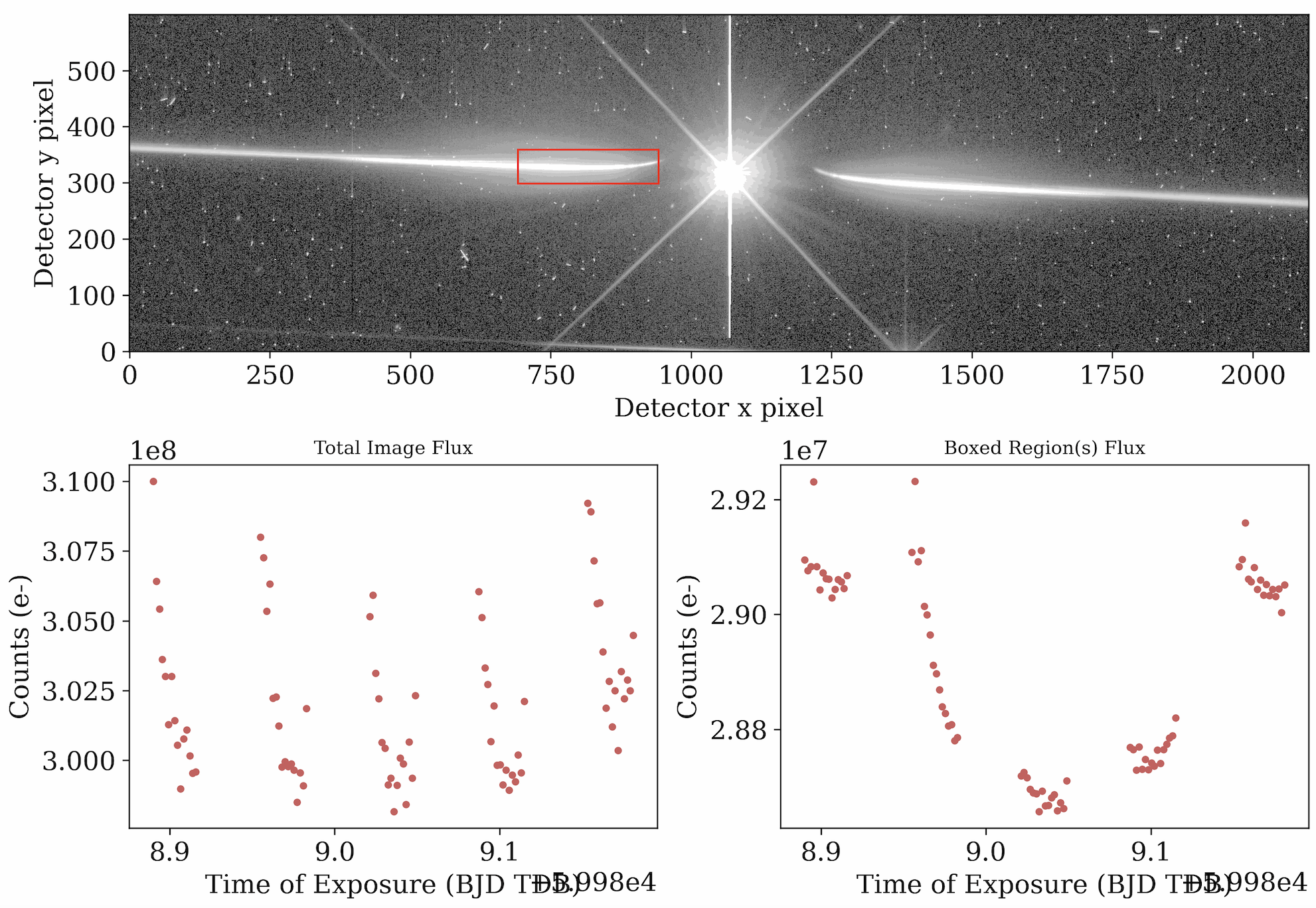
Last frame of quicklookup.gif file from visit 12 of HST-GO 17183, with a clear transit visible in the bottom right plot.
4.2. The outputs of Stage 1
Stage 1 handles data reduction, and outputs a lot of diagnostic plots we can use to assess whether our reduction strategy is appropriate. Open the outputs/stage_1/demo/plots/ folder or inspect your terminal/notebook outputs and take a look at the following plots:
CR_location.png plots the location of all pixels flagged as a cosmic ray in any frame in any orbit. CR_location_frameX.png shows the cosmic rays flagged in individual frame number X. Both of these plots show us that our cosmic ray rejection routine successfully targeted cosmic rays without overcorrecting the data.
bkg_values_corners.png shows us the estimated background value in each frame. bkg_before_subtraction.png and bkg_after_subtraction.png plot the first frame of the observation before and after the estimated background value was subtracted.
target_location_in_direct_image.png plots the updated position of the target star in the direct image, and 0th_tracking_frameX.png shows the 0th order position in frame X. The plotted positions match the center of the star’s PSF very well, ensuring our wavelength calibration in Stage 2 will succeed.
0th_order_x_displacement.png and 0th_order_y_displacement.png show the position of the bright 0th order in the data frames over time. Small sub-pixel shifts in pointing can introduce systematic trends into our extracted 1D spectral time-series, but by measuring these shifts now we can correct for them later.
Stage 1 also outputs a revised quicklookup.gif that we can compare to our Stage 0 gif to see how the frames have changed after reduction. We also receive a similar gif showing the data quality array, which shows the pixels in each frame that were flagged for data quality issues during reduction (e.g. cosmic rays caught by temporal rejection, hot pixels caught by spatial rejection, etc.).
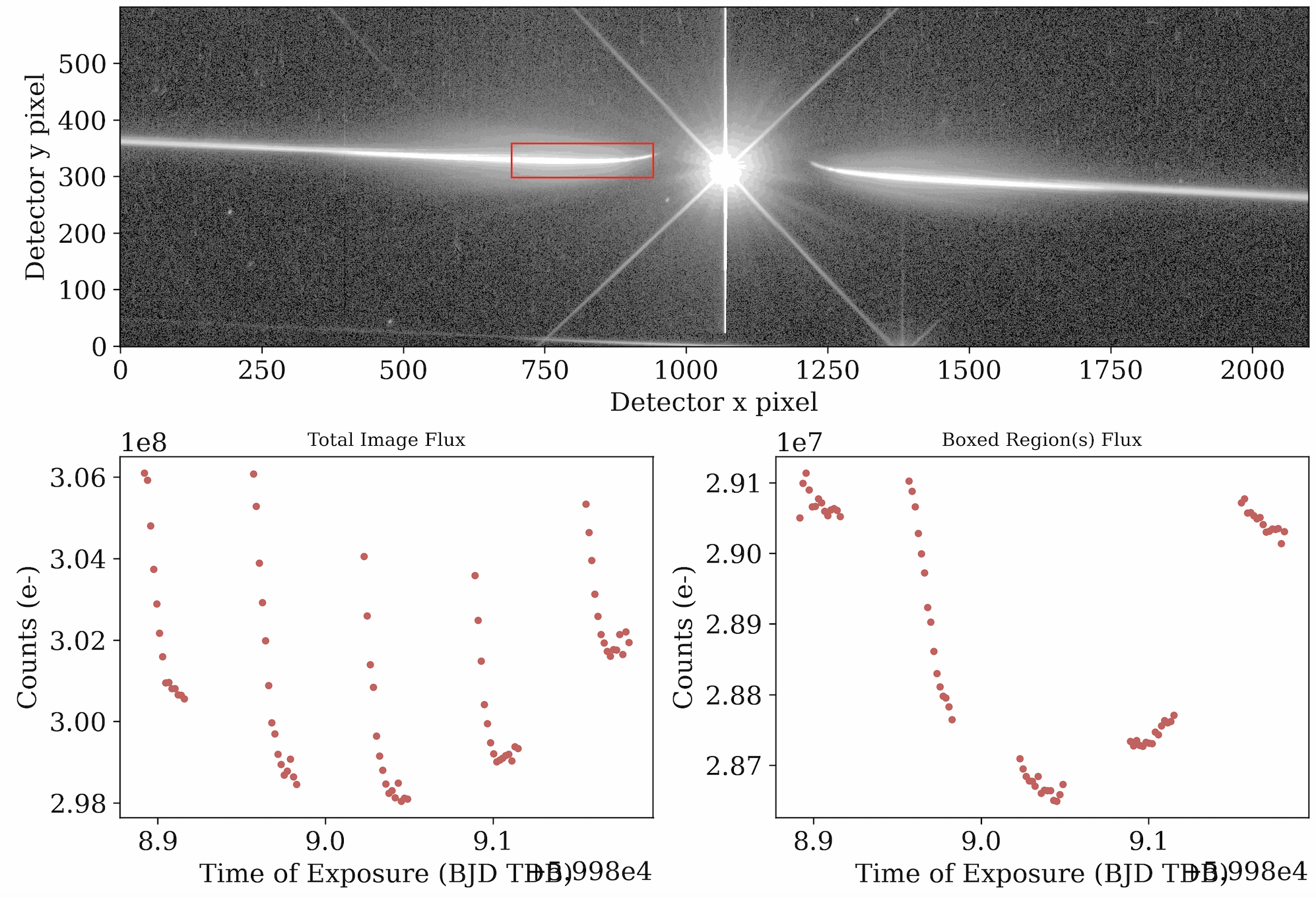
The last frame of the quick lookup after cleaning. The data frames are free of cosmic rays and hot pixels with a smooth background (top), while the transit light curve shows greatly reduced scatter (bottom right). |
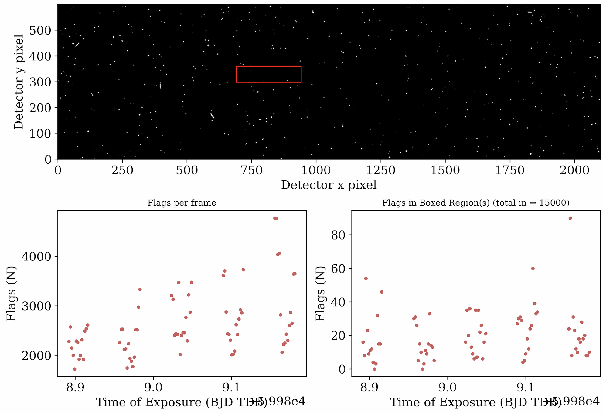
The data quality array for the same frame. White marks pixels flagged as outliers. The total flags in the frame (bottom left) and the flags in the boxed region (right) are also displayed; neither exceeds 5% of the data. |
4.3. The outputs of Stage 2
Stage 2 extracts the 1D spectral time series from our reduced data frame, and likewise produces lots of diagnostic plots for our use. Open the outputs/stage_2/demo/plots/ folder or inspect your terminal/notebook outputs and take a look at the following plots:
calibration_+1.png and calibration_-1.png show the
grismconfcalibrated positions of the +1 and -1 order traces. If your calibration was successful, these should fall right along the middle of the brightest curves on either side of the 0th order.aperture_+1.png and aperture_-1.png likewise show the calibration solution as well as the upper and lower bounds of the the aperture for extraction. A good aperture is wide enough to encompass the trace and its wings without pulling in too much background noise.
cross_corr_order+1.png, cross_corr_order-1.png, trace_crossdisp_profiles_order+1.png, and trace_crossdisp_profiles_order-1.png show the displacements estimated from cross-correlating the traces. These can also be used to detrend systematics.
1Dspec_order+1.png and 1Dspec_order-1.png show the first frame’s 1D spectrum for each order. 2Dspec_order+1.png and 2Dspec_order-1.png plot the 1D spectra in every frame over time as a 2D map. 1Dspec_order+1.gif and 1Dspec_order-1.gif plays all extracted 1D spectra for each order as a gif. All of these plots can be used to assess the quality of the extracted spectra, including looking for uncorrected cosmic rays or systematic signals. In this dataset, a strong systematic can be seen in the -1 order at 400 nm.
rawwlc_order+1.png and rawwlc_order-1.png show the white light curves obtained by summing all 1D spectra across all wavelengths. These light curves should be clean and with good signal-to-noise ratio, with minimal systematic patterns and no spurious points from e.g. cosmic rays.
The 1D spectra for each order will be output to specs_+1.nc and specs_-1.nc which can be opened and manipulated with the xarray package, documented here. These are the final science products on which you would perform your analyses. For example, the script below can be used to generate a plot of the white and spectroscopic light curves from this observation:
import numpy as np
import xarray as xr
import matplotlib.pyplot as plt

#define plotting parameters
plt.rc('font', family='serif')
plt.rc('xtick', labelsize=14)
plt.rc('ytick', labelsize=14)
plt.rc('axes', labelsize=14)
plt.rc('legend',**{'fontsize':11})


specs = xr.open_dataset('output/outputs/stage2/demo/specs_+1.nc')

# Get the timestamps of exposures.
exp_time = specs.exp_time

# Open the 1D spectral time series and its uncertainties
spectrum = specs.spec    # has shape exp_time x wavelengths
errors = specs.spec_err  # same shape as above

# Open the grismconf wavelength solution
wavelengths = specs.wave

# Create a plot.
layout = """
    AAA
    BCD
"""
fig, ax = plt.subplot_mosaic(layout,figsize=(16,5),sharey=True)
plt.subplots_adjust(wspace=0,hspace=0.3)

# Make a white light curve.
wlc = np.sum(spectrum,axis=1)
wle = np.sqrt(np.sum(np.square(errors),axis=1))
wle /= np.median(wlc)
wlc /= np.median(wlc)
ax['A'].errorbar(exp_time,wlc,yerr=wle,capsize=3,markersize=3,marker='o',color='k',ls='none')
ax['A'].set_xlabel('')
ax['A'].set_ylabel('Flux [a.u.]')
ax['A'].tick_params(which='both',axis='both',direction='in')
ax['A'].set_title("White Light Curve")

# Make a red, green, and blue light curve.
for wavelength,color,letter in zip((2000,4000,6000),
                                   ('blue','green','red'),
                                   ('B','C','D')):
    ok = (wavelengths>=wavelength) & (wavelengths<=wavelength+2000)
    slc = np.sum(spectrum[:,ok],axis=1)
    sle = np.sqrt(np.sum(np.square(errors[:,ok]),axis=1))
    sle /= np.median(slc)
    slc /= np.median(slc)

    ax[letter].errorbar(exp_time,slc,yerr=sle,capsize=3,markersize=3,marker='o',color=color,ls='none')
    ax[letter].set_xlabel('Exposure Time [MJD]')
    if letter == 'B':
        ax[letter].set_ylabel('Flux [a.u.]')
    ax[letter].tick_params(which='both',axis='both',direction='in')
    ax[letter].set_title(f'{wavelength+1000} AA')
plt.savefig('light_curves.png',dpi=300,bbox_inches='tight')
plt.close()
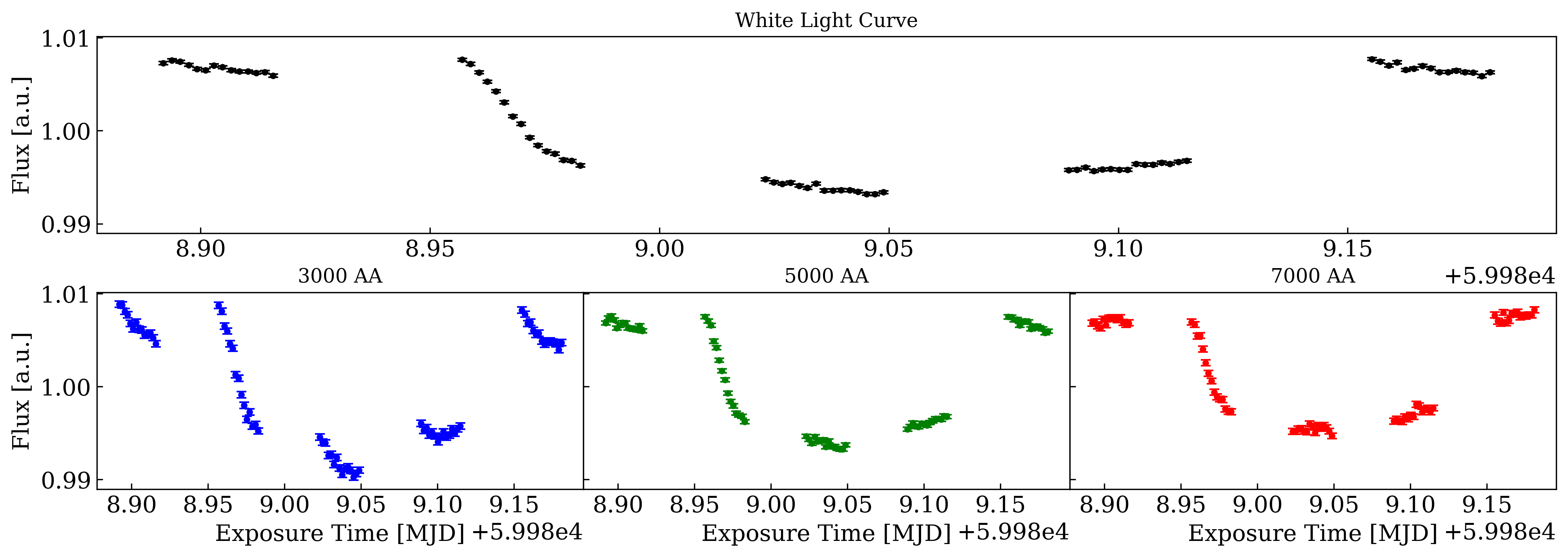
The white light curve (top) and spectroscopic light curves (bottom) created from our HUSTLE-tools reduction of a transit of WASP-127 b observed in HST-GO 17183. Note the increasing transit depth at shorter wavelengths.
5. What next?
That’s it for the quick start! You are now ready to start running HUSTLE-tools on your own data! If you want to learn more about how to adjust .hustle configuration files and operate each stage, head over to the Tutorials page!