Stage 2: Extraction

Prefer Jupyter notebooks? A .ipynb of this tutorial is also available on GitHub!

NOTE: Make sure you ran Stage 0: Data Handling and Stage 1: Reduction before attempting this stage!

Now that the data are clean, we want to extract the 1D spectral time series from the traces. HUSTLE-tools Stage 2 calibrates the wavelength solution of your cleaned data to extract the spectrum from 200 to 800 nm. This tutorial will walk you through this process.

Creating the Stage 2 configuration file

The first step is to create the configuration file that will guide the execution of Stage 2. Create a folder to store the configuration file in, e.g. configs/. Then create configs/stage_2_input_config.hustle and populate it with the following template:

# HUSTLE-tools config file for launching Stage 2: Extraction

# Setup for Stage 2
toplevel_dir    './files'                                   # Directory where your current project files are stored. This folder should contain the specimages/, directimages/, etc. folders with your data as well as the outputs folder.
input_run       'run_1'                                     # Str. This is the name of the Stage 1 run you want to load.
output_run      'run_1'                                     # Str. This is the name to save the current run to. It can be anything that does not contain spaces or special characters (e.g. $, %, @, etc.).
verbose         2                                           # Int from 0 to 2. 0 = print nothing. 1 = print some statements. 2 = print every action.
show_plots      2                                           # Int from 0 to 2. 0 = show nothing. 1 = show some plots. 2 = show all plots.
save_plots      2                                           # Int from 0 to 2. 0 = save nothing. 1 = save some plots. 2 = save all plots.

# Step 1: Read in the data

# Step 2: Trace configuration
path_to_cal     './'                                        # Str. The absolute path to the .conf file used by GRISMCONF for the chip your data were taken on.
traces_to_conf  ('+1','-1')                                 # Lst of str. The traces you want to configure and extraction from.
refine_fit      True                                        # Bool. If True, uses Gaussian fitting to refine the trace solution.

# Step 3: Time And Relative Detrending In Space (TARDIS)
do_tardis       True                                        # Bool. Whether to use TARDIS to clean the timeseries. Useful for low-cadence datasets where Stage 1 cleaning methods are prone to missing trace-striking cosmic rays.
tardis_sigma    [5.0,3.5]                                   # list of float. The sigmas to reject outliers at. One sigma per window value is needed.
flux_threshold  1000                                        # float. The e-/s counts value above which this method will be used. Method fails if there is insufficient flux to detect trends with, so keep this at least as high as the median wing flux value.
tardis_window   [10,5]                                      # list of int. Median time-series trends will be measured using pixels +/- window columns away from target pixel.
tardis_replace  'tseries'                                   # str. If 'tseries', uses median time-series trends to replace outliers. If 'median', uses pixel's median value in time to replace outliers.

# Step 4: 1D spectral extraction
method          'box'                                       # Str. Options are 'box' (draw a box around the trace and sum without weights) or 'optimal' (weight using Horne 1986 methods).
correct_zero    False                                       # Bool. Whether to model the contaminating 0th order and subtract it from your data during extraction. Sometimes works, sometimes just adds lots of scatter.
sens_correction False                                       # Bool. Whether to correct for the G280's changing sensitivity as a function of wavelength. Since absolute calibrated spectra aren't needed in exoplanetary sciences, you can skip this safely.
mask_objs       [[0,0,0],]                                  # List of lists. If there are background objects in your planned aperture, mask them here. Each entry is (x,y,radius).

# Step 4a: Box extraction parameters
determine_hw    True                                        # Bool. If True, automatically determines preferred half-width for each order by minimizing out-of-transit/eclipse residuals.
indices         ([0,10],[-10,-1])                           # Lst of lsts of int. If determine_hw, these are the indices used to estimate the out-of-transit/eclipse residuals.
halfwidths_box  (12,12)                                     # Lst of ints. The half-width of extraction aperture to use for each order. Input here is ignored if 'determine_hw' is True.

# Step 4b: Optimum extraction parameters
aperture_type   'median'                                    # Str. Type of aperture to draw. Options are 'median', 'polyfit', 'smooth', or 'curved_poly'.
halfwidths_opt  (12,12)                                     # Lst of ints. The half-width of extraction aperture to use for each order. For optimum extraction, you should make this big (>12 pixels at least). There is no 'preferred' half-width in optimum extraction due to the weights.

# Step 5: 1D spectral cleaning and aligning
outlier_sigma   3.5                                         # Float. Sigma at which to reject spectral outliers in time. Outliers are replaced with median of timeseries. Enter False to skip this step.
align           True                                        # Bool. If True, uses cross-correlation to align spectra to keep wavelength solution consistent.
apply_align     True                                        # Bool. If False while Align is True, then the wavelength shifts will be measured but the spectra will not be shifted. Useful for diagnosing align efficacy.

# ENDPARSE

Let’s break down each of these steps to make sure we understand what we can tune in this stage.

Setup for Stage 2

You can customize the toplevel_dir folder to be any name you like as long as you use the same folder name for all stages. You will likely run multiple reductions of the data as you explore different cleaning strategies, which will each be output to their own Stage 1 output_run folder. Now in Stage 2, we can adjust the input_run parameter to select which of these Stage 1 outputs we want to receive as our Stage 2 input, allowing you to pick your best reduction to work with for this stage. As with Stage 1, you may also want to run Stage 2 multiple times to test different extraction apertures and methods. To keep each run separate so that no files get overwritten, you can adjust the output_run variable each time you run Stage 2. This will cause the outputs to go to a subfolder with the name toplevel_dir/outputs/stage_2/output_run. The verbose, show_plots, and save_plots keys respectively control the level of detail in the statements printed by the pipeline while it executes, the number of plots opened in the terminal or .ipynb notebook cell you are running the script in, and the number of plots saved out to .png or .gif files to be reviewed at any time after execution.

Step 1: Read in the data

At this step, the pipeline reads in the chosen Stage 1 outputs, which at present has no variables for you to adjust.

Step 2: Trace configuration

HUSTLE-tools uses grismconf, a package developed by Pirzkal & Ryan 2017, to assign the field-dependent wavelength solution to the traces you want to extract. If you followed the instructions on the Installation page, you should have downloaded a set of WFC3/UVIS configuration files which grismconf will use to determine the wavelength solution for each order based on the target position you located in Stage 0 and optionally refined in Stage 1. Depending on which of the two WFC3/UVIS CCD chips you collected your observations on, you must supply the path_to_cal variable with the absolute path to either your local UVIS_G280_CCD1_V2.conf file for chip 1, or your local UVIS_G280_CCD2_V2.conf file for chip 2. It is recommended by Wakeford et al. 2020 to use chip 2 for WFC3/UVIS observations because it is more stable than chip 1. Your observations are also most likely collected on chip 2, which you can confirm by opening the .fits files and checking the CCDCHIP keyword of the [SCI] header, as shown below.

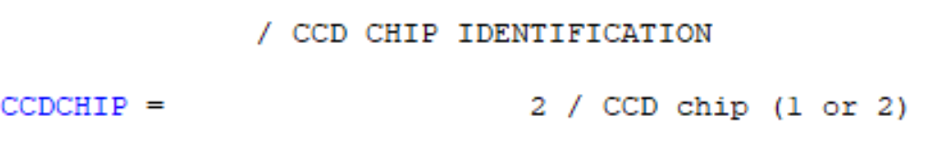
[SCI] header info showing the CCD chip number stored in the CCDCHIP keyword.

grismconf supports extraction of both the positive (higher throughput, dispersed to left) orders and the negative (lower throughput, dispersed to right) orders, with support for up to the 4th order trace. All traces are extractable, but note that higher order traces have less flux and are more contaminated, which can make reliable extraction more challenging. You can specify which traces you want to extract by supplying the sign and order of each trace in the traces_to_conf variable, e.g. by supplying this variable as (“+1”,”-1”) you can request to extract the positive and negative 1st-order traces.

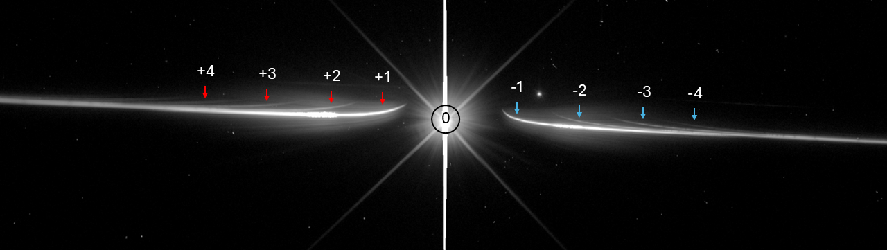
A WFC3/UVIS G280 data frame showing the 0th order (middle), all extractable positive orders (left), and all extractable negative orders (right).

Shifts in the trace position over time can affect the wavelength solution, which is determined from the static direct photometric image taken at the observation start. You can refine the trace solution by setting refine_fit to True to allow the trace solution to be updated in each frame.

Step 3: Time And Relative Detrending In Space (TARDIS)

HST UVIS/G280 traces contain very strong systematics as documented in e.g. Wakeford et al. 2016. These systematics can be strong enough to mask cosmic ray hits even when the cosmic ray is on the order of 10% or more of the pixel’s median flux. Stage 1 HUSTLE-tools may miss these rays entirely. The Time And Relative Detrending In Space (TARDIS) routine was developed specfically to identify trace-striking cosmic rays hidden by systematic trends. Set do_tardis to True to execute this routine. You can perform multiple rounds of TARDIS at different thresholds of outlier rejection by supplying a list of floats to tardis_sigma. The flux_threshold parameter ensures TARDIS does not operate on non-trace pixels with low flux. Each round of TARDIS can also use a different window size across which to measure local systematic trends through the tardis_window list. Smaller windows with lower thresholds of rejection effectively clean the curved UV portion of the trace, while larger windows and higher thresholds operate on the straight IR portion of the trace. Set tardis_replace to ‘tseries’ to replace outliers with the locally-measured time-series trend, or set it to ‘median’ to use the pixel’s median value in time.

Step 4: 1D spectral extraction

The core of Stage 2 is the extraction of the 1D spectral time series from each trace requested. HUSTLE-tools offers two methods of aperture weighting which you set by the method variable: box and optimal. Additional subsections below detail variables unique to each method. Regardless of method used, you can also adjust several steps designed to deal with sources of contamination in G280 data. correct_zero can be set to True to prompt HUSTLE-tools to build an empirical model of the 0th order wing flux, which is dispersed widely across the G280 frame and which can especially dilute transit depths in the UV and blue-optical wavelengths. G280 orders are overlapped, causing the transit depth in each order to be diluted where it is intercepted by other orders. Setting subtract_contam to True prompts HUSTLE-tools to model the wavelength-dependent dilution affecting each other due to other orders intercepting it, and to subtract off contaminating flux from these other orders. If absolute spectra are desired, you can set sens_correction to True to correct for the G280’s wavelength-dependent sensitivity, returning the intrinsic flux of the observed source. Near-field objects such as stars or galaxies can sometimes enter the extraction aperture if the telescope’s position angle is just so. To mask these objects, supply mask_objs with a list of the x-y position of the field object as well as the radius in pixels out to which a circular mask will be drawn over the field object.

Step 4a: Box extraction parameters

The box method of extraction simply draws an unweighted aperture around the trace and sums the flux of all pixels within. The scatter in the extracted 1D spectrum depends sensitively on the halfwidth of this box aperture. Too narrow an aperture will exclude trace flux from extraction and lower the signal-to-noise, while too wide an aperture will sum up noisy background pixels that do not contribute any source flux. You can set determine_hw to True to allow HUSTLE-tools to determine an extraction aperture halfwidth that minimizes the scatter in the out-of-transit residuals, and thereby maximizes the signal-to-noise ratio of your 1D spectra. If you use this method, set the out-of-transit indices of your data with indices. You can also set the halfwidth for each order yourself using the halfwidths_box variable.

Step 4b: Optimum extraction parameters

The optimal extraction method detailed by Horne 1986 uses variance to weight each pixel within the extraction aperture, assigning stronger weight to bright pixels and weaker weight to dim, noisy pixels. The linked paper details multiple methods of developing the weights applied to each pixel, such as by using the median image over time or constructing polynomial fits to each row and/or column. You can specify which aperture model you want to use with the aperture_type variable. Because of the weights, there is no preferred halfwidth for extraction as there is in standard box extraction. You can still specify the aperture halfwidths with the halfwidths_opt variable, and ideally for optimal extraction these halfwidths should be large.

Step 5: 1D spectral cleaning and aligning

Even after all of the cleaning processes run in Stage 1, outliers may still find their way into your extracted 1D spectral time series. You can reject temporal outliers in each extracted channel using the outlier_sigma parameter. Additionally, drift in the dispersion direction over time may cause the grismconf wavelength solution to slowly drift away from the data. You can cross-correlate the drifting spectra by setting align to True, and re-align the spectra by setting apply_align to True.

Running Stage 2

Now that you understand what each variable does, edit your config file as you like. With the configuration file created and stored in configs/stage_2_input_config.hustle, create a simple .py or .ipynb script with the following contents:

from hustle_tools import run_pipeline

config_files_dir = "configs"
stages = (2,)

run_pipeline(config_files_dir, stages)

Then execute this script to run Stage 2! The output in your cell should look similar to the output shown below, where we have used HST-GO 17183 (PI: Hannah Wakeford), visit 12, target WASP-127 as an example:

Extracting standard spectra... Progress:: 100%|██████████████████████████████████████████████████████████████████████████████████████| 74/74 [00:02<00:00, 36.55it/s]
Aligning spectra in order +1... Progress:: 74it [00:00, 139.23it/s]
Computing profile displacements... Progress:: 100%|████████████████████████████████████████████████████████████████████████████████| 421/421 [00:28<00:00, 14.63it/s]
MovieWriter ffmpeg unavailable; using Pillow instead.
Extracting standard spectra... Progress:: 100%|██████████████████████████████████████████████████████████████████████████████████████| 74/74 [00:01<00:00, 58.90it/s]
Aligning spectra in order -1... Progress:: 74it [00:00, 153.17it/s]
Computing profile displacements... Progress:: 100%|████████████████████████████████████████████████████████████████████████████████| 390/390 [00:26<00:00, 14.52it/s]
MovieWriter ffmpeg unavailable; using Pillow instead.
Writing config file for Stage 2...
Config file written.

Assessing Stage 2’s success

Stage 2 is also a fairly customizable stage and has many diagnostics to look over.

Diagnostic 1: Calibration and apertures acquired traces

The calibration and aperture plots should show that Stage 2 located the correct traces, and that the apertures encompass the entirety of the orders you have chosen to extract from. Below we show aperture plots including the trace position calibration for the +1 and -1 traces of a V~10 star with an effective temperature of 5600 K, observed by HST-GO 17183.

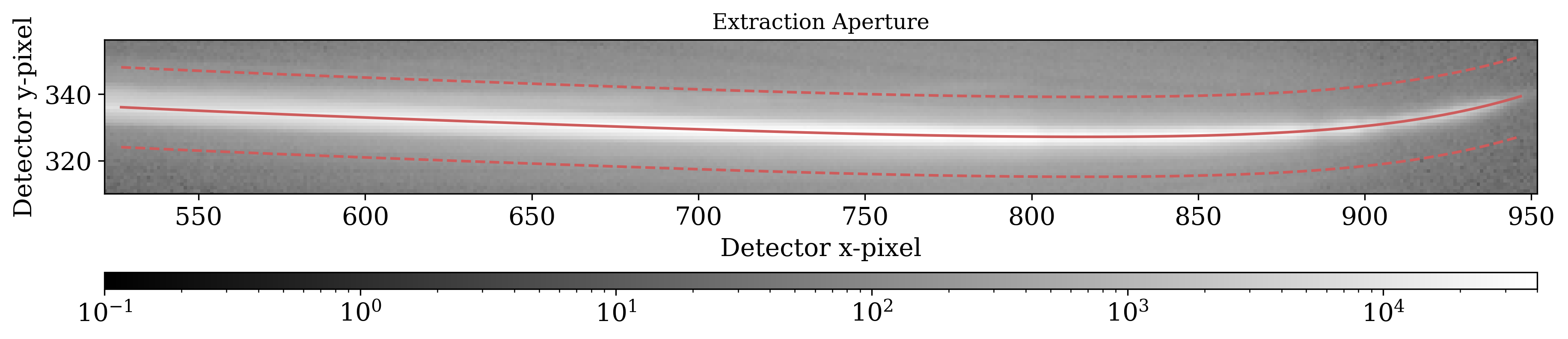
Aperture (dashed lines) encasing the +1 trace with a halfwidth of 12 pixels. The calibration solution (solid line) traces the dispersed spectra to a sub-pixel accuracy.

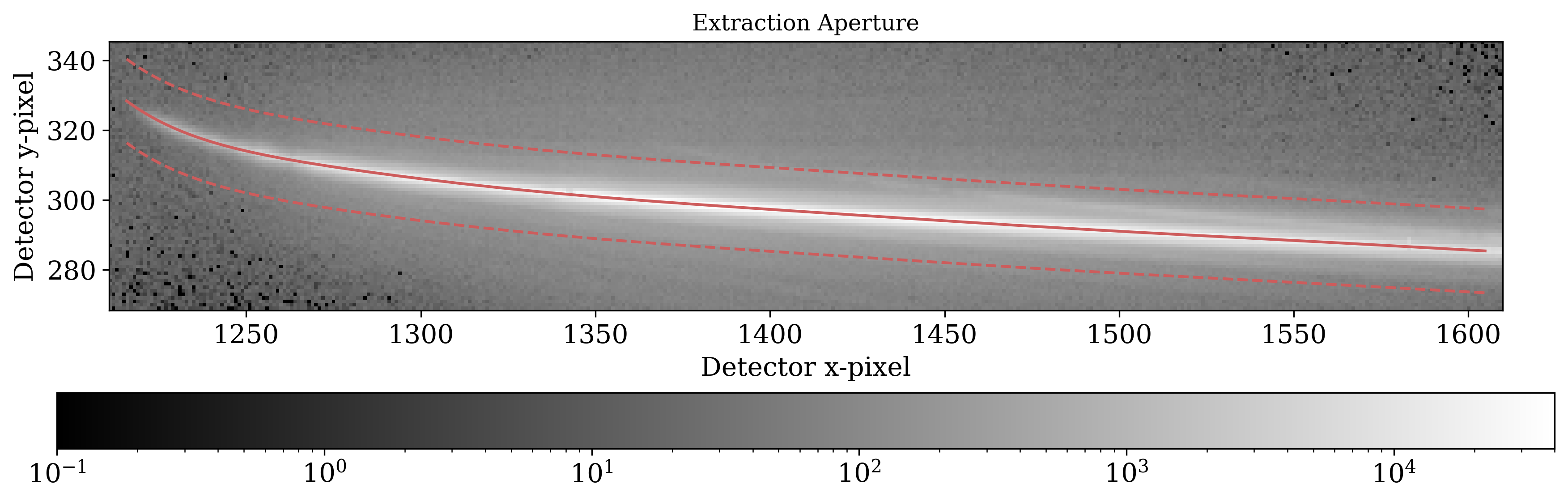
Aperture (dashed lines) encasing the -1 trace with a halfwidth of 12 pixels. The calibration solution (solid line) traces the dispersed spectra to a sub-pixel accuracy.

We additionally show calibration plots for the traces from another HST-GO 17183 observation for a V~7 star at an effective temperature of 8000 K. Note that unlike the data for the cooler star, the higher orders in this data are readily visible. Self-contamination from overlapping orders poses a significant challenge in processing datasets with low-V, high-T stars! For most stars, the higher orders will be barely resolved and self-contamination contributes much less error than the photon noise limit, so self-contamination treatment is often unnecessary.

Below we show orders +1 through +4, which can all be extracted albeit with increasing self-contamination.

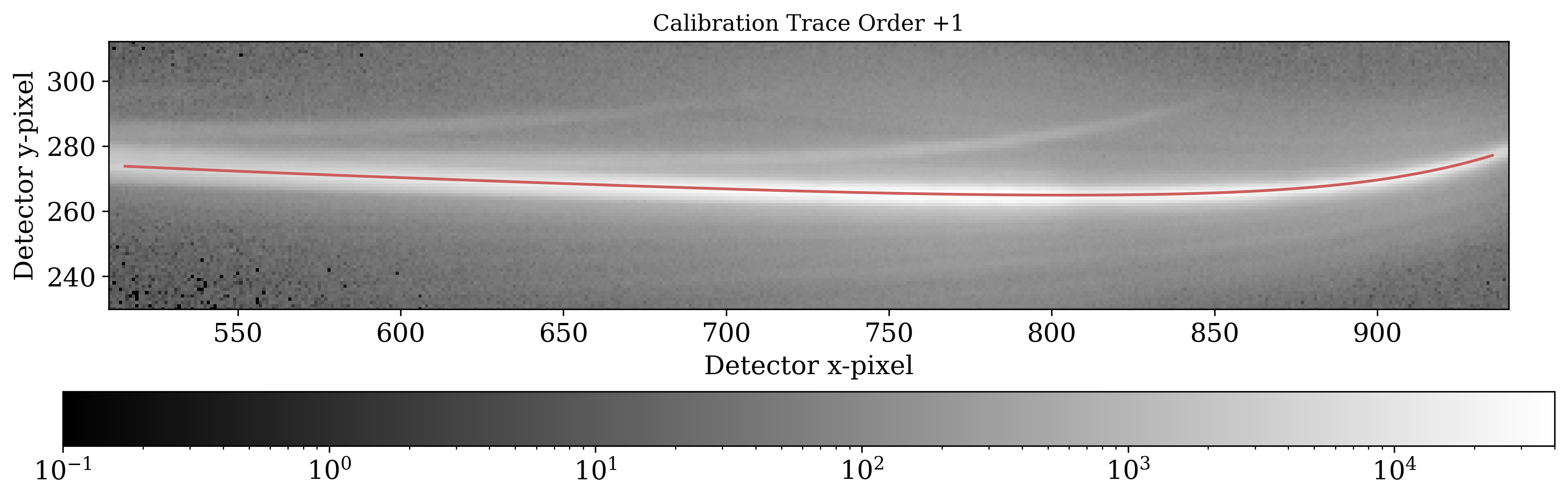
+1 order.

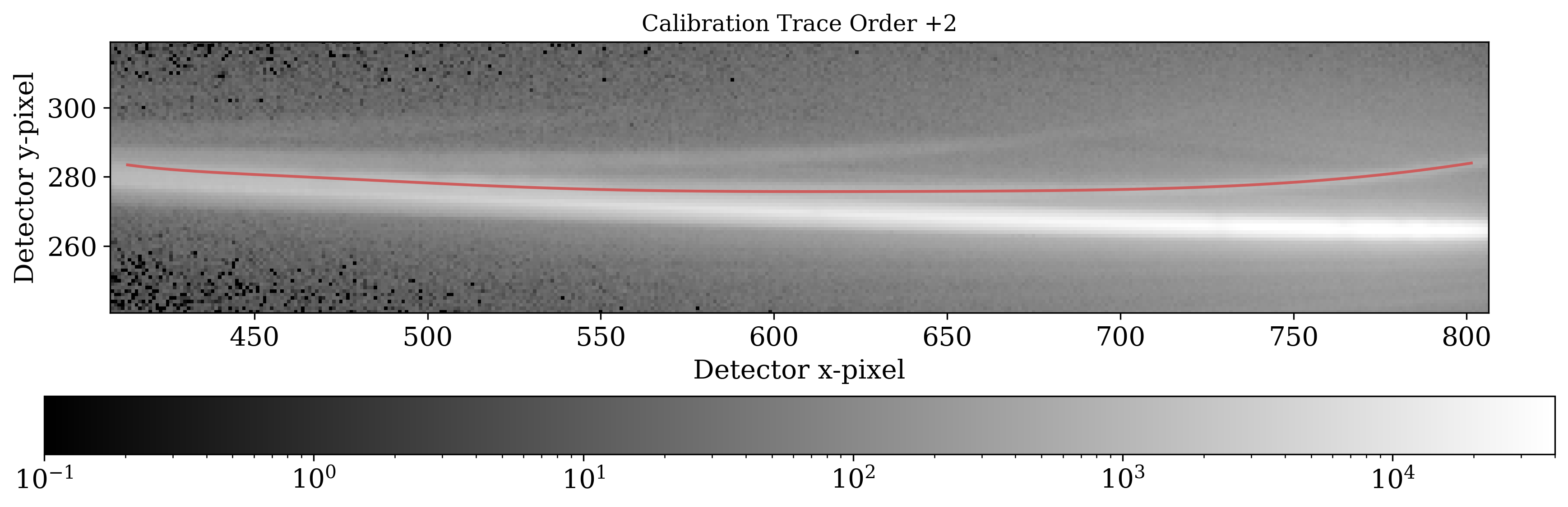
+2 order.

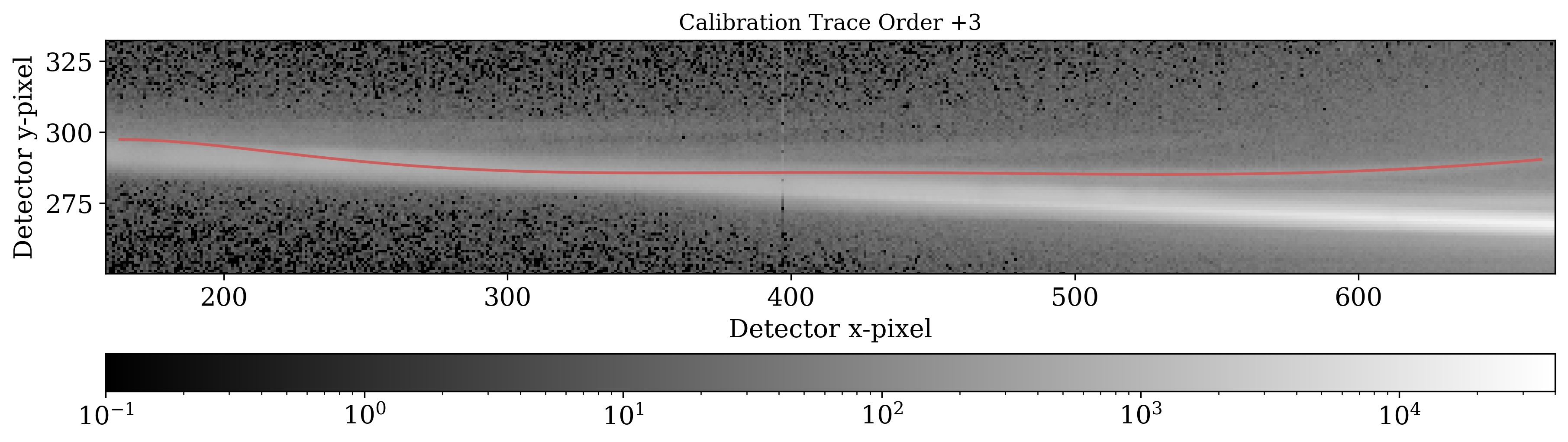
+3 order.

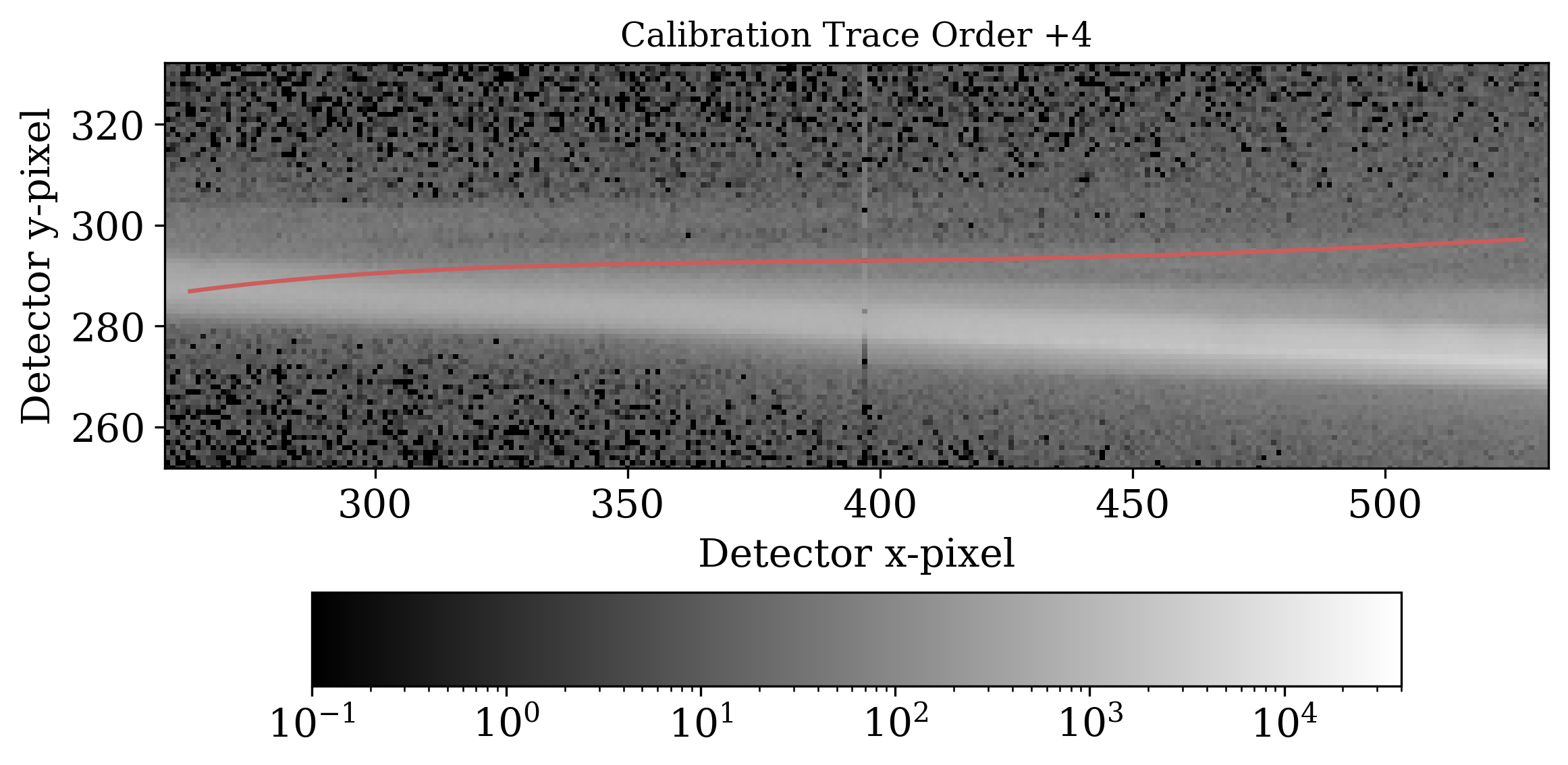
+4 order.

Below we show orders -1 through -4, which can all be extracted albeit with increasing self-contamination.

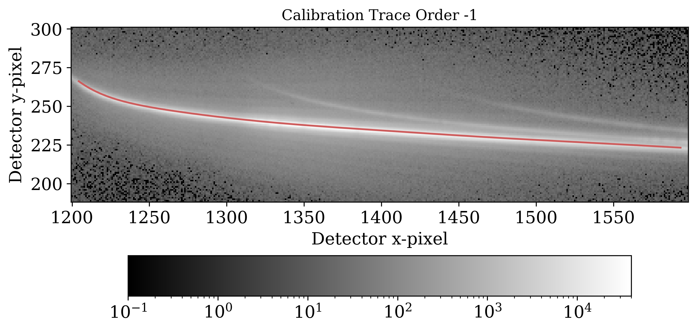
-1 order.

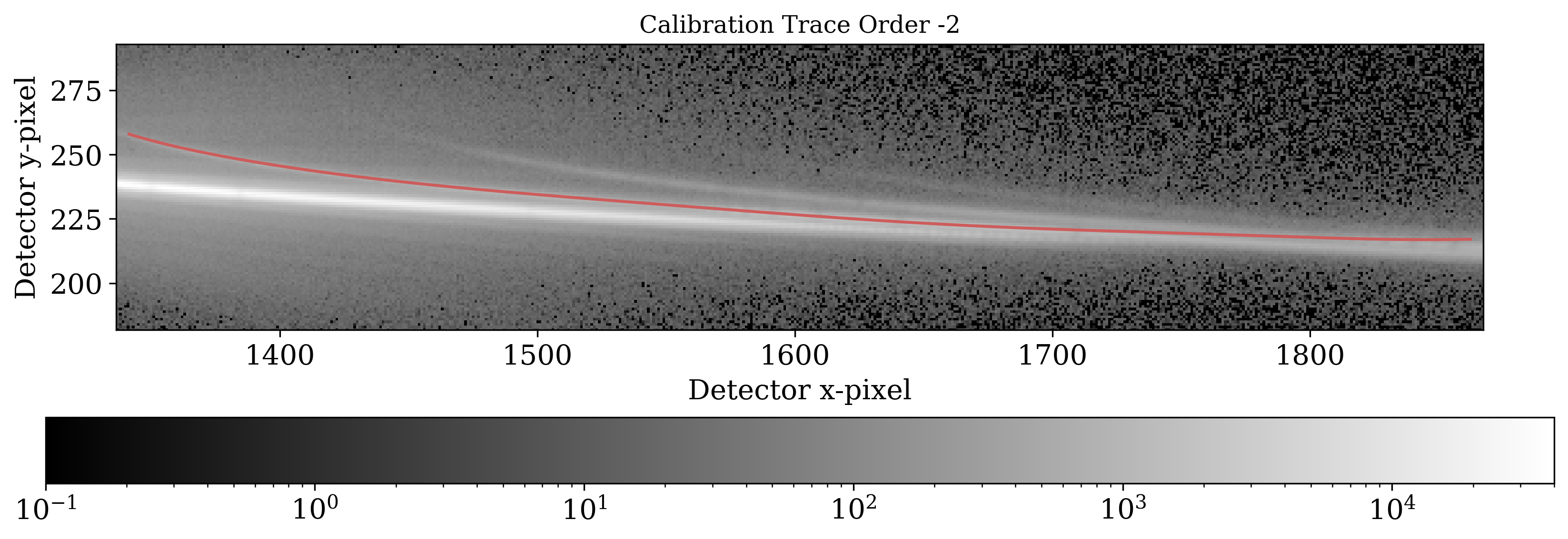
-2 order.

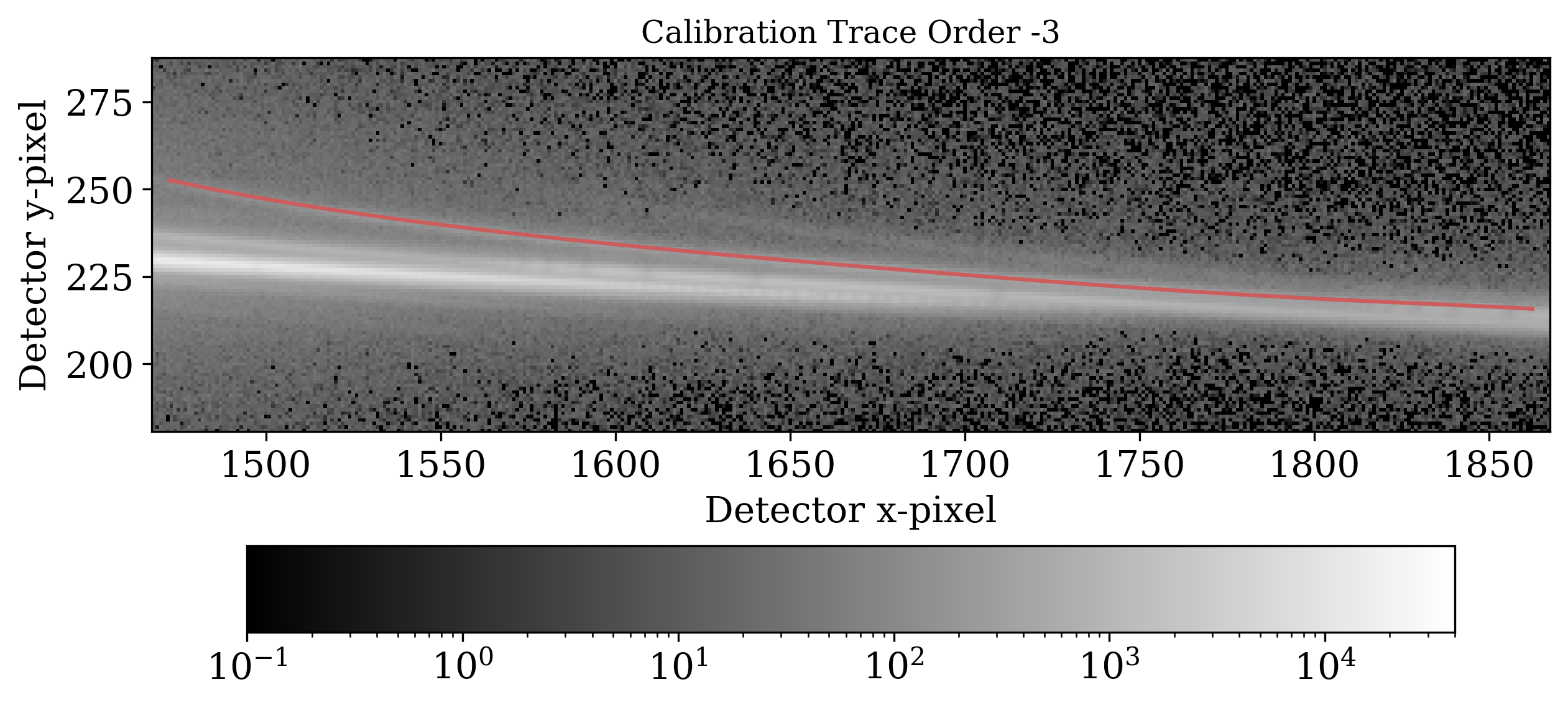
-3 order.

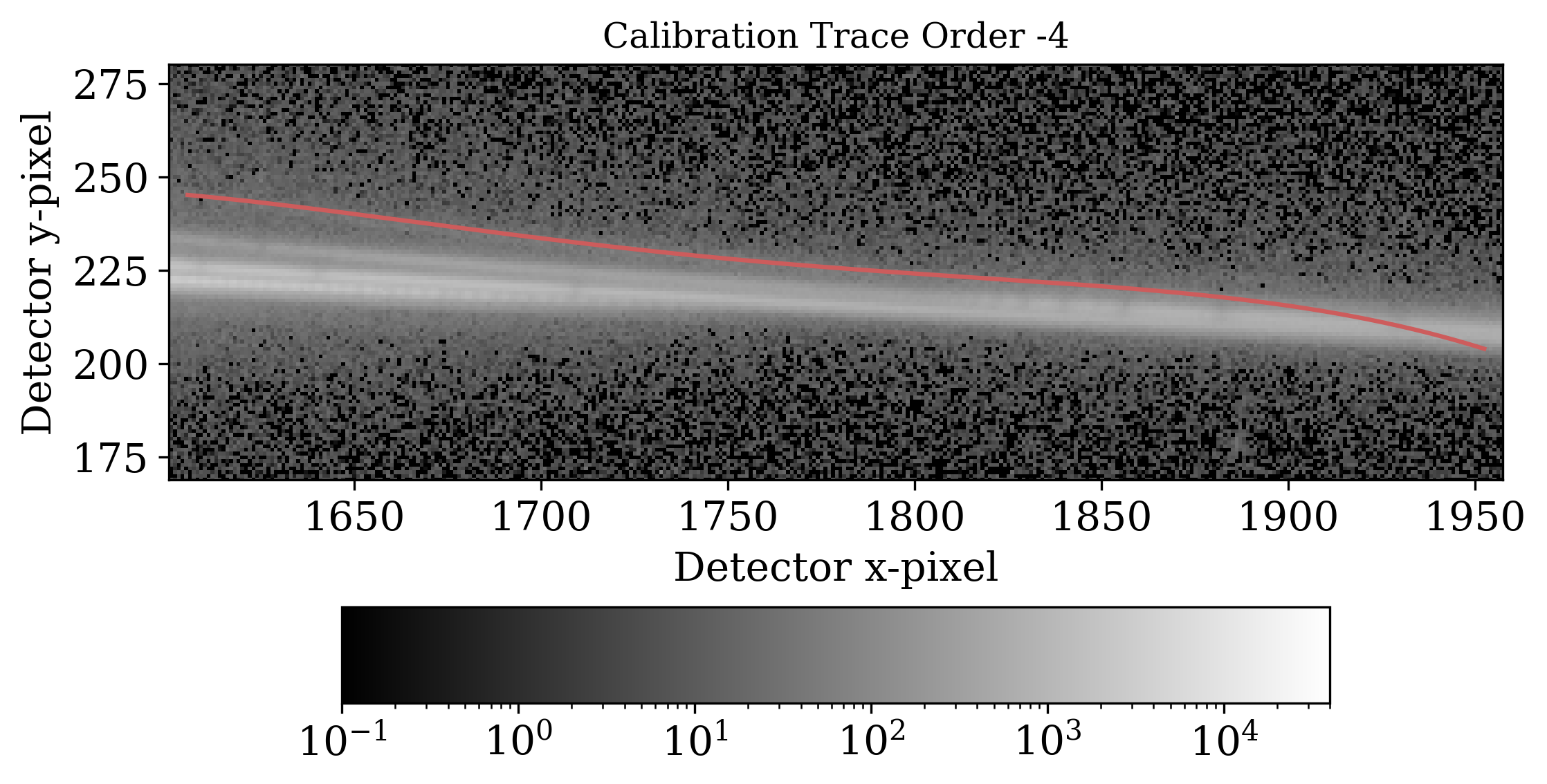
-4 order.

Diagnostic 2: 1D spectral time series of source

The extracted 1D spectral time series should be consistent with the source spectrum expected (e.g. if your target is an A star, you should be able to see Balmer absorption lines in the spectrum centered at the appropriate wavelengths), and the 1D spectrum gif should show no cosmic ray spikes, drift over time, or reduction process artifacts (e.g. rapid variations or dramatic changes in flux in certain channels which can arise from hot/cold/dead pixels, an up-and-down jitteriness that might be the result of bad background subtraction, etc.).

We show an example +1 1D spectral time series from HST-GO 17183 below.

The 1D spectral time series for the +1 order.

We show an example -1 1D spectral time series from HST-GO 17183 below.

The 1D spectral time series for the -1 order.

Diagnostic 3: Comparison between orders

The extracted orders should be reasonably consistent with each other, where their wavelength ranges overlap. Some minor differences should be expected due to order throughput variations, but the overall shape and features should be comparable. Below we show the overplotted +1 and -1 spectra of WASP-127 from HST-GO 17183.

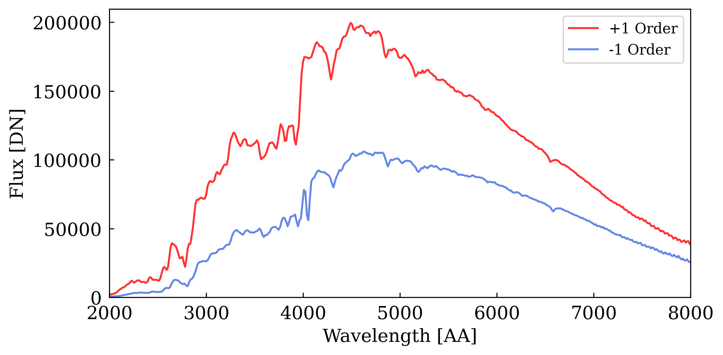
The median +1 (red) and -1 (blue) 1D spectra. Apart from a scaling factor, the two spectra are otherwise largely consistent in terms of shape and features.

Diagnostic 4: Stage 2 displacement consistency with Stage 1

The cross-correlation dispersion and cross-dispersion shifts should be reasonably consistent with each other, and with the x-y shifts measured in the background stars (if available) in Stage 1. The shifts may be somewhat less consistent with the 0th order motions, especially in the y direction, due to saturation and bloom affecting 0th order tracking. We show the cross-correlation shifts for both the dispersion and cross-dispersion directions for the +1 1D spectral time series of WASP-127 from HST-GO 17183, overplotted with the x-y shifts measured from the 0th order.

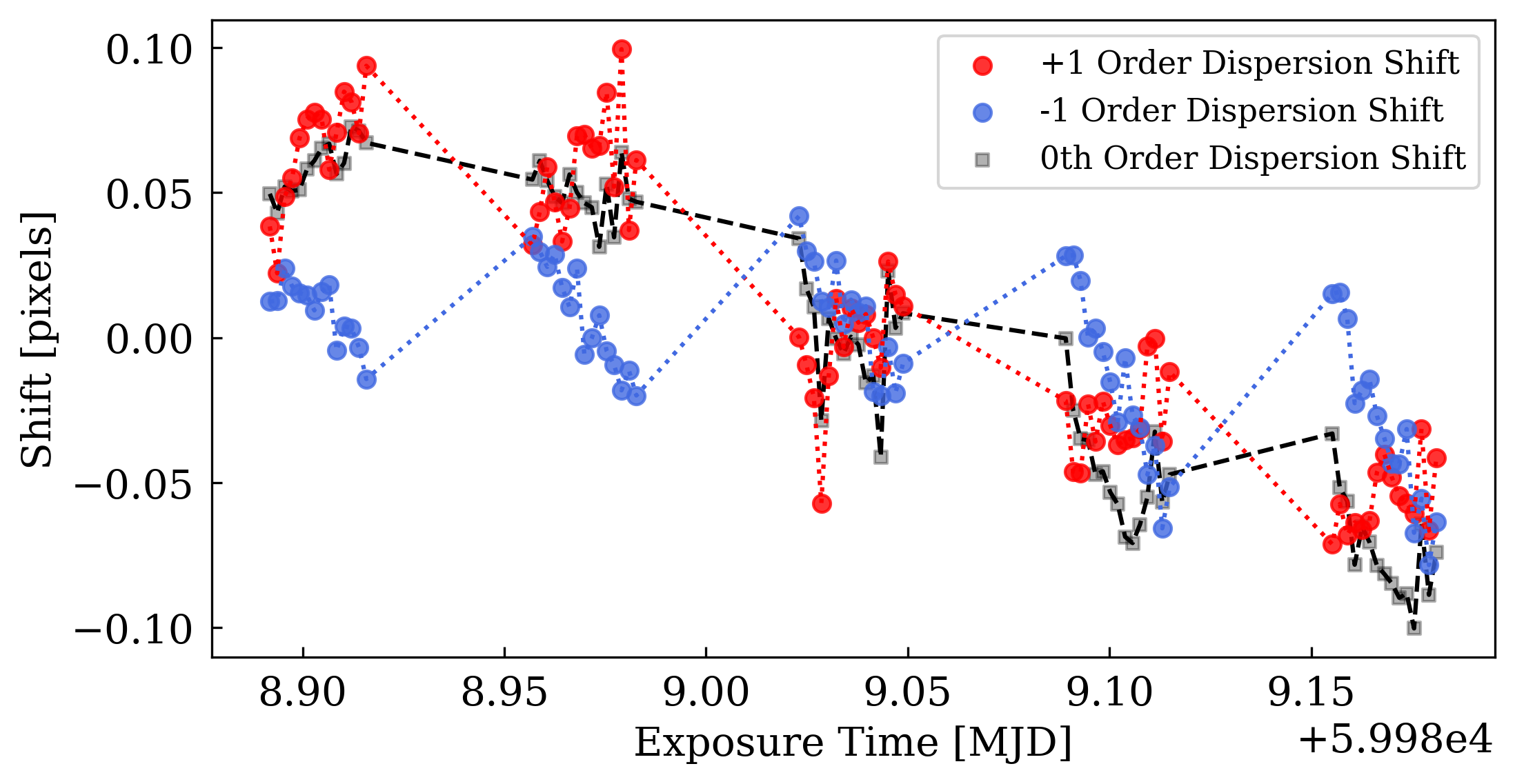
Dispersion shifts of the +1 and -1 orders measured with cross-correlation. As the traces are mirrors of each other in the dispersion direction, the +1 and -1 shifts are mirrored.

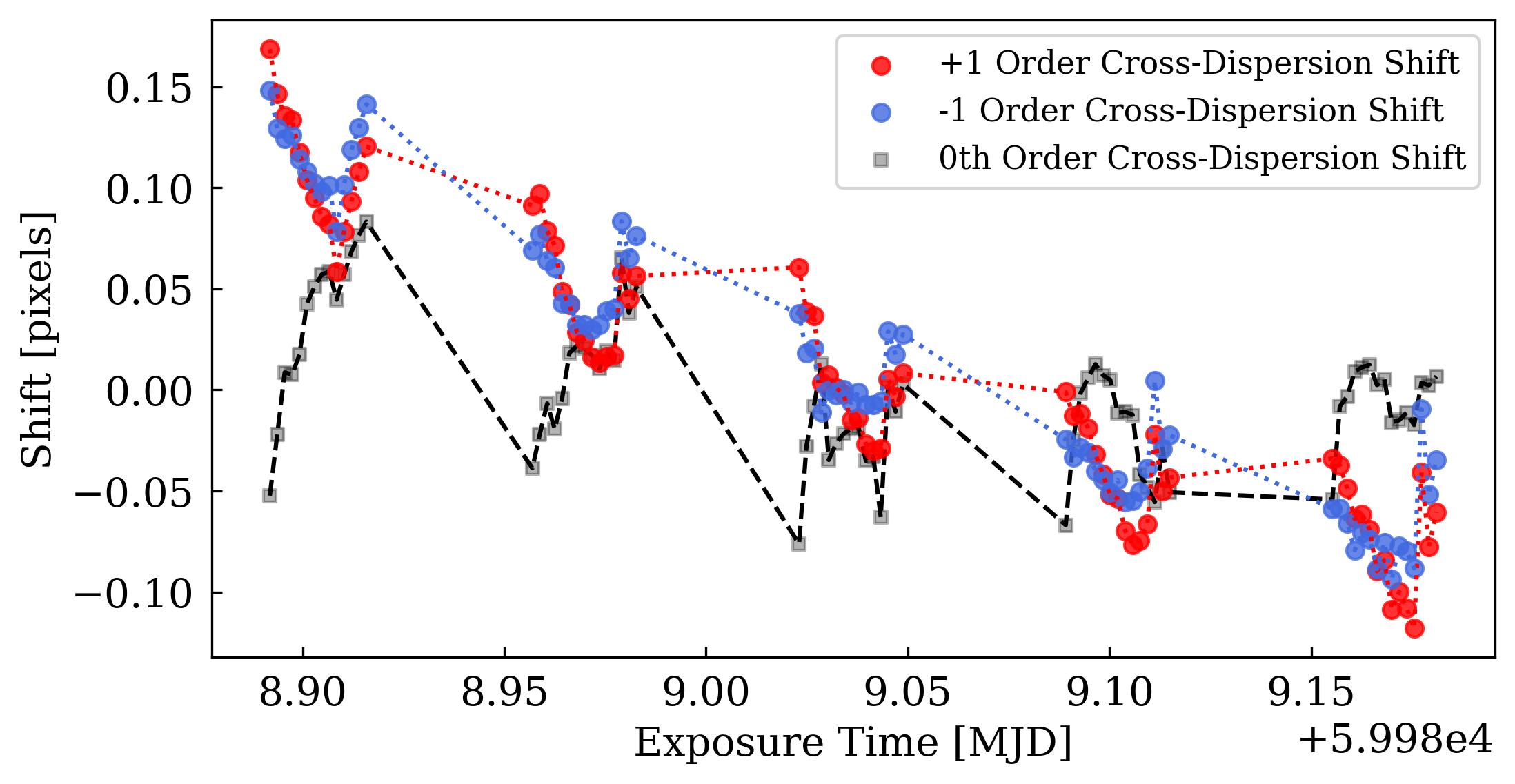
Cross-dispersion shifts of the +1 and -1 orders measured with cross-correlation. As the traces are symmetric in the cross-dispersion direction, the +1 and -1 shifts are alike.

Diagnostic 5: Raw white light curves show expected shape and quality

The extracted raw white light curves for each order should clearly show the event you expect to observe, with the level of scatter that you expect. Bear in mind that some systematics should still be present at this stage - these can be treated using a variety of methods including systematic marginalisation (Wakeford et al. 2016) and jitter decorrelation (Sing et al. 2019). We show the raw white light curves for the +1 and -1 order of WASP-127 below.

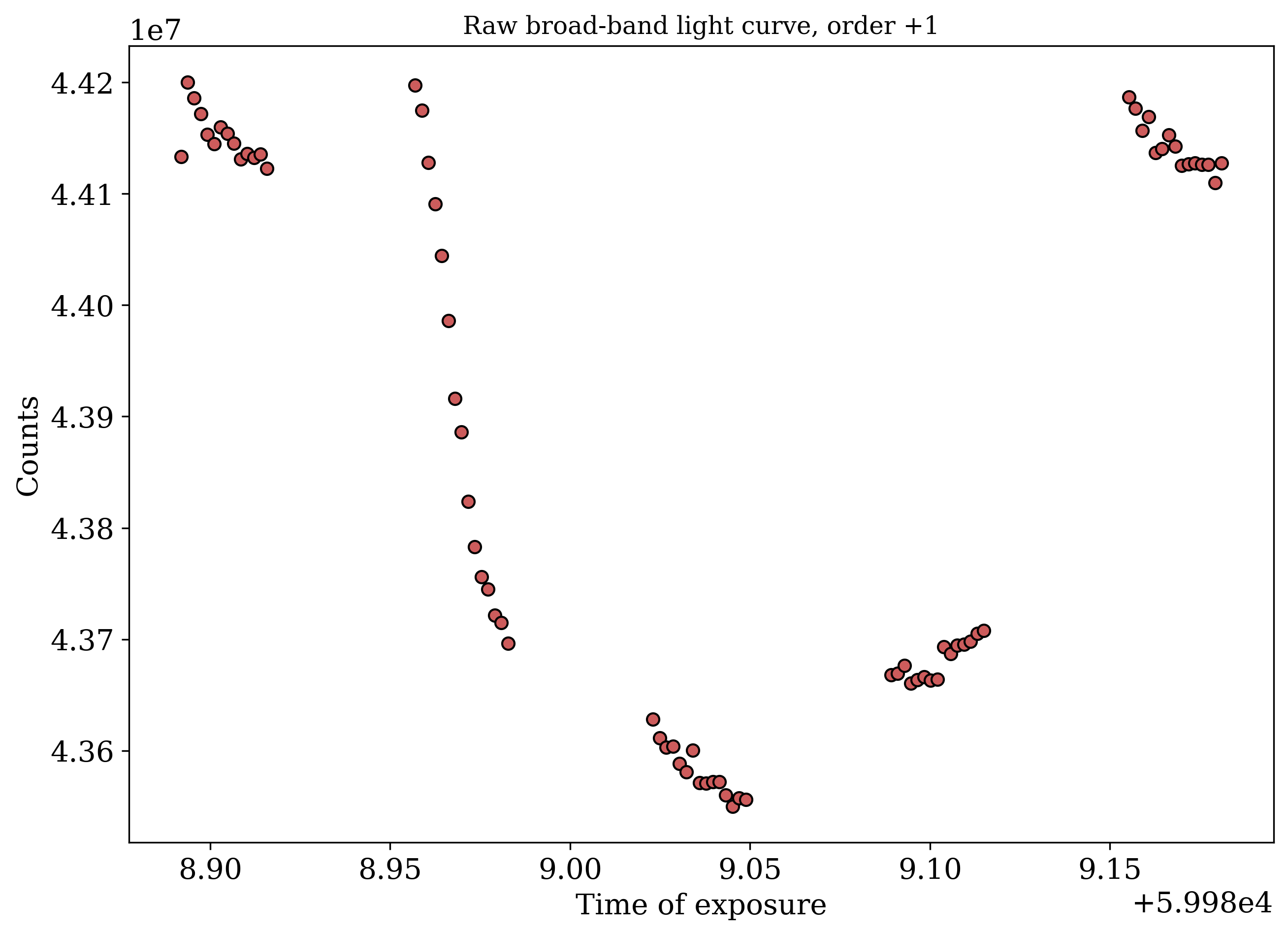
The raw white light curve from the +1 order. While systematics are present that skew each orbit’s shape, the scatter is reasonably consistent with expectations.

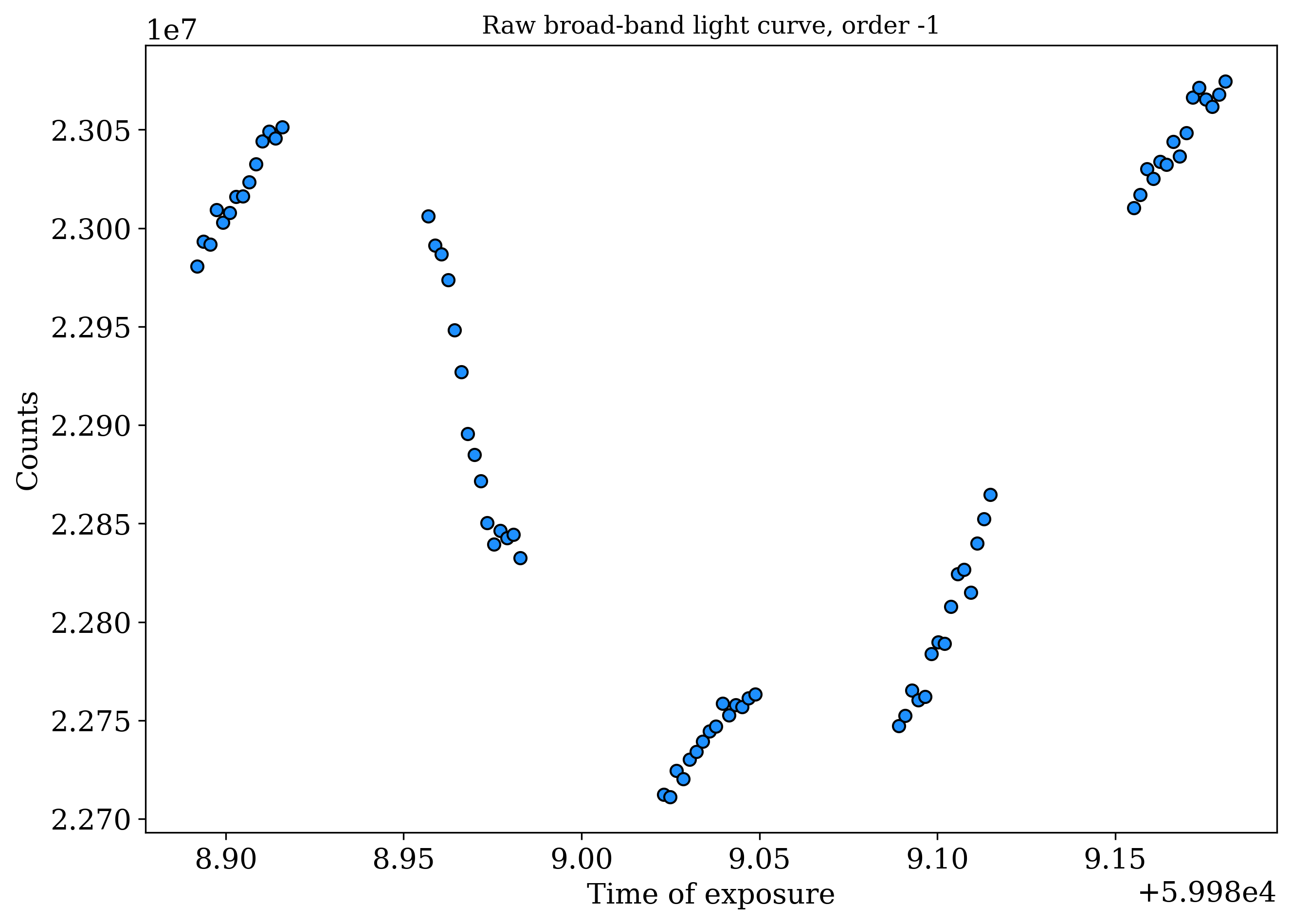
The raw white light curve from the -1 order. Compared to the brighter +1 order, the dimmer -1 order light curve shows greater scatter and systematics.